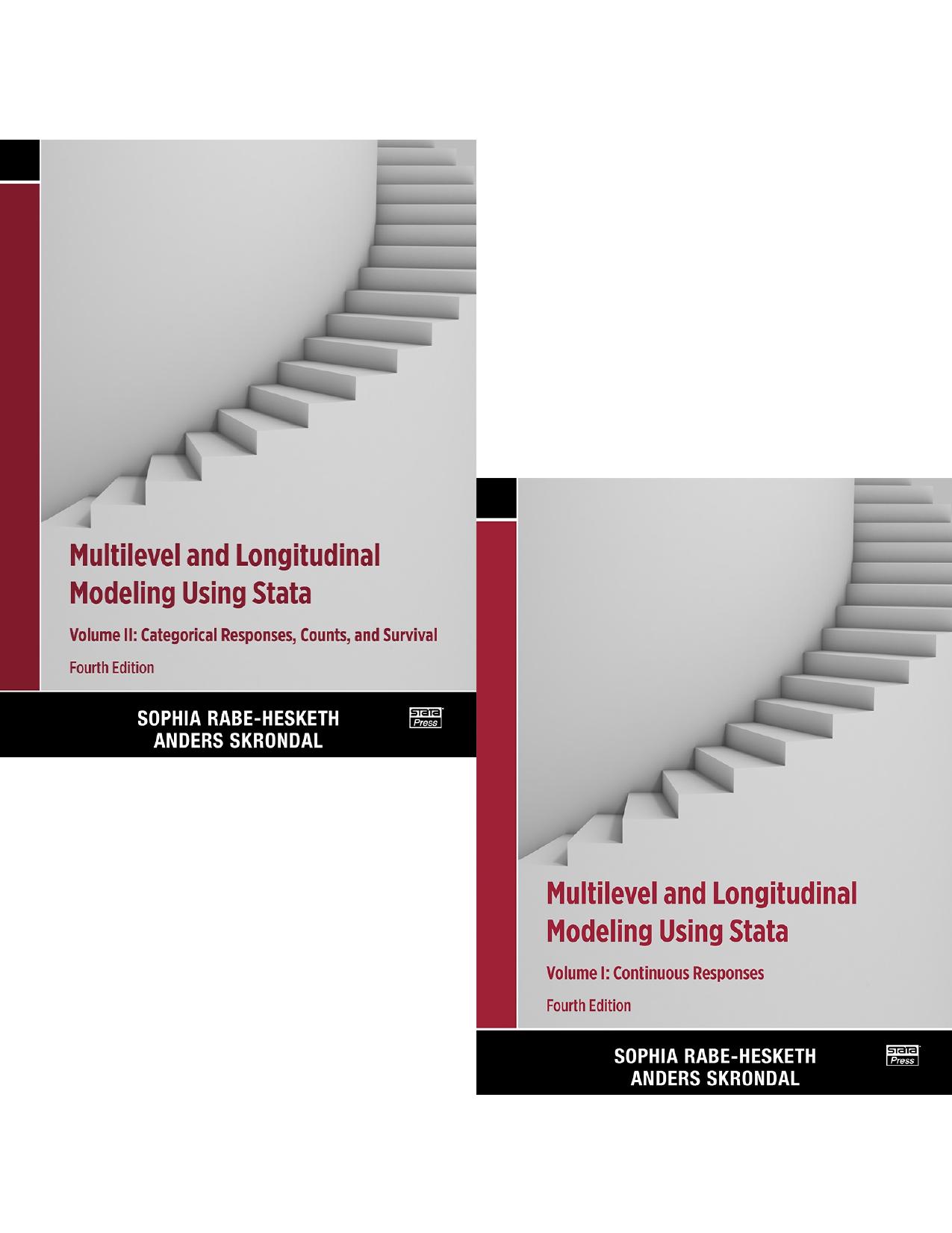
Multilevel and Longitudinal Modeling Using Stata 4th Edition by Sophia Rabe Hesketh,Anders Skrondal 1597181366 9781597181365
$70.00 Original price was: $70.00.$35.00Current price is: $35.00.
Instant download Multilevel and Longitudinal Modeling Using Stata Fourth Edition Volumes I and II Sophia Rabe Hesketh;Anders Skrondal; after payment
Multilevel and Longitudinal Modeling Using Stata 4th Edition by Sophia Rabe Hesketh,Anders Skrondal – Ebook PDF Instant Download/Delivery:1597181366,9781597181365
Full dowload Multilevel and Longitudinal Modeling Using Stata 4th Edition after payment

Product details:
ISBN 10:1597181366
ISBN 13:9781597181365
Author:Sophia Rabe Hesketh,Anders Skrondal
Multilevel and Longitudinal Modeling Using Stata, Fourth Edition, is a complete resource for learning to model data in which observations are grouped―whether those groups are formed by a nesting structure, such as children nested in classrooms, or formed by repeated observations on the same individuals. This text introduces random-effects models, fixed-effects models, mixed-effects models, marginal models, dynamic models, and growth-curve models, all of which account for the grouped nature of these types of data. As Rabe-Hesketh and Skrondal introduce each model, they explain when the model is useful, its assumptions, how to fit and evaluate the model using Stata, and how to interpret the results. With this comprehensive coverage, researchers who need to apply multilevel models will find this book to be the perfect companion. It is also the ideal text for courses in multilevel modeling because it provides examples from a variety of disciplines as well as end-of-chapter exercises that allow students to practice newly learned material.
The book comprises two volumes. Volume I focuses on linear models for continuous outcomes, while volume II focuses on generalized linear models for binary, ordinal, count, and other types of outcomes.
Multilevel and Longitudinal Modeling Using Stata 4th Table of contents:
1.2 Is there gender discrimination in faculty salaries?
1.3 Independent-samples t test
1.4 One-way analysis of variance
1.5 Simple linear regression
1.6 Dummy variables
1.7 Multiple linear regression
1.8 Interactions
1.9 Dummy variables for more than two groups
1.10 Other types of interactions
1.10.2 Interaction between continuous covariates
1.11 Nonlinear effects
1.12 Residual diagnostics
1.13 Causal and noncausal interpretations of regression coefficients
1.13.2 Regression as structural model
1.14 Summary and further reading
1.15 Exercises
2.2 How reliable are peak-expiratory-flow measurements?
2.3 Inspecting within-subject dependence
2.4 The variance-components model
2.4.2 Path diagram
2.4.3 Between-subject heterogeneity
2.4.4 Within-subject dependence
Intraclass correlation versus Pearson correlation
2.5 Estimation using Stata
2.5.2 Using xtreg
2.5.3 Using mixed
2.6 Hypothesis tests and confidence intervals
2.6.2 Hypothesis test and confidence interval for the between-cluster variance
Score test
F test
Confidence interval
2.7 Model as data-generating mechanism
2.8 Fixed versus random effects
2.9 Crossed versus nested effects
2.10 Parameter estimation
Distributional assumptions
2.10.2 Different estimation methods
2.10.3 Inference for β
Estimate: Unbalanced case
2.11 Assigning values to the random intercepts
Implementation via the mean total residual
2.11.2 Empirical Bayes prediction
2.11.3 Empirical Bayes standard errors
Diagnostic standard errors
Accounting for uncertainty in <span id="MathJax-Element-1-Frame" class="MathJax" style="box-sizing: border-box; display: inline; font-style: normal; font-weight: normal; line-height: normal; font-size: 14.6667px; font-size-adjust: none; text-indent: 0px; text-align: left; text-transform: none; letter-spacing: normal; word-spacing: normal; overflow-wrap: normal; white-space: nowrap; float: none; direction: ltr; max-width: none; max-height: none; min-width: 0px; min-height: 0px; border: 0px; padding: 0px; margin: 0px; position: relative;" tabindex="0" role="presentation" data-mathml="β^”>β^β^
2.11.4 Bayesian interpretation of REML estimation and prediction
2.12 Summary and further reading
2.13 Exercises
3.2 Does smoking during pregnancy affect birthweight?
3.3 The linear random-intercept model with covariates
3.3.2 Model assumptions
3.3.3 Mean structure
3.3.4 Residual covariance structure
3.3.5 Graphical illustration of random-intercept model
3.4 Estimation using Stata
3.4.2 Using mixed
3.5 Coefficients of determination or variance explained
3.6 Hypothesis tests and confidence intervals
3.6.2 Joint hypothesis tests for several regression coefficients
3.6.3 Predicted means and confidence intervals
3.6.4 Hypothesis test for random-intercept variance
3.7 Between and within effects of level-1 covariates
3.7.2 Within-mother effects
3.7.3 Relations among estimators
3.7.4 Level-2 endogeneity and cluster-level confounding
3.7.5 Allowing for different within and between effects
3.7.6 Robust Hausman test
3.8 Fixed versus random effects revisited
3.9 Assigning values to random effects: Residual diagnostics
3.10 More on statistical inference
Feasible generalized least squares (FGLS)
ML by iterative GLS (IGLS)
ML by Newton–Raphson and Fisher scoring
ML by the expectation-maximization (EM) algorithm
REML
3.10.2 Consequences of using standard regression modeling for clustered data
Purely within-cluster covariate
3.10.3 Power and sample-size determination
Purely within-cluster covariate
3.11 Summary and further reading
3.12 Exercises
4.2 How effective are different schools?
4.3 Separate linear regressions for each school
4.4 Specification and interpretation of a random-coefficient model
4.4.2 Interpretation of the random-effects variances and covariances
4.5 Estimation using mixed
4.5.2 Random-coefficient model
4.6 Testing the slope variance
4.7 Interpretation of estimates
4.8 Assigning values to the random intercepts and slopes
4.8.2 Empirical Bayes prediction
4.8.3 Model visualization
4.8.4 Residual diagnostics
4.8.5 Inferences for individual schools
4.9 Two-stage model formulation
4.10 Some warnings about random-coefficient models
4.10.2 Many random coefficients
4.10.3 Convergence problems
4.10.4 Lack of identification
4.11 Summary and further reading
4.12 Exercises
5.2 Random-effects approach: No endogeneity
5.3 Fixed-effects approach: Level-2 endogeneity
Subject dummies
5.3.2 Hausman test
5.3.3 Mundlak approach and robust Hausman test
5.3.4 First-differencing
5.4 Difference-in-differences and repeated-measures ANOVA
5.4.2 Repeated-measures ANOVA
5.5 Subject-specific coefficients
5.5.2 Fixed-coefficient model: Level-2 endogeneity
5.6 Hausman–Taylor: Level-2 endogeneity for level-1 and level-2 covariates
5.7 Instrumental-variable methods: Level-1 (and level-2) endogeneity
5.7.2 Conventional fixed-effects approach
5.7.3 Fixed-effects IV estimator
5.7.4 Random-effects IV estimator
5.7.5 More Hausman tests
5.8 Dynamic models
5.8.2 Dynamic model with subject-specific intercepts
5.9 Missing data and dropout
5.9 Summary and further reading
5.10 Exercises
6.2 Mean structure
6.3 Covariance structures
6.3.2 Random-intercept or compound symmetric/exchangeable structure
6.3.3 Random-coefficient structure
6.3.4 Autoregressive and exponential structures
6.3.5 Moving-average residual structure
6.3.6 Banded and Toeplitz structures
6.4 Hybrid and complex marginal models
6.4.2 Heteroskedastic level-1 residuals over occasions
6.4.3 Heteroskedastic level-1 residuals over groups
6.4.4 Different covariance matrices over groups
6.5 Comparing the fit of marginal models
6.6 Generalized estimating equations (GEE)
6.7 Marginal modeling with few units and many occasions
6.7.2 Marginal modeling for long panels
6.7.3 Fitting marginal models for long panels in Stata
6.8 Summary and further reading
6.9 Exercises
7.2 How do children grow?
7.3 Models for nonlinear growth
Predicting the mean trajectory
Predicting trajectories for individual children
7.3.2 Piecewise linear models
Predicting the mean trajectory
7.4 Two-stage model formulation and cross-level interaction
7.5 Heteroskedasticity
7.5.2 Heteroskedasticity at level 2
7.6 How does reading improve from kindergarten through third grade?
7.7 Growth-curve model as a structural equation model
7.7.2 Estimation using mixed
7.8 Summary and further reading
7.9 Exercises
8.2 Do peak-expiratory-flow measurements vary between methods within subjects?
8.3 Inspecting sources of variability
8.4 Three-level variance-components models
8.5 Different types of intraclass correlation
8.6 Estimation using mixed
8.7 Empirical Bayes prediction
8.8 Testing variance components
8.9 Crossed versus nested random effects revisited
8.10 Does nutrition affect cognitive development of Kenyan children?
8.11 Describing and plotting three-level data
8.11.2 Level-1 variables
8.11.3 Level-2 variables
8.11.4 Level-3 variables
8.11.5 Plotting growth trajectories
8.12 Three-level random-intercept model
8.12.2 Model specification: Three-stage formulation
8.12.3 Estimation using mixed
8.13 Three-level random-coefficient models
8.13.2 Random coefficient at the child and school levels
8.14 Residual diagnostics and predictions
8.15 Summary and further reading
8.16 Exercises
9.2 How does investment depend on expected profit and capital stock?
9.3 A two-way error-components model
9.3.2 Residual variances, covariances, and intraclass correlations
Cross-sectional correlations
9.3.3 Estimation using mixed
9.3.4 Prediction
9.4 How much do primary and secondary schools affect attainment at age 16?
9.5 Data structure
9.6 Additive crossed random-effects model
9.6.2 Intraclass correlations
9.6.3 Estimation using mixed
9.7 Crossed random-effects model with random interaction
9.7.2 Intraclass correlations
9.7.3 Estimation using mixed
9.7.4 Testing variance components
9.7.5 Some diagnostics
9.8 A trick requiring fewer random effects
9.9 Summary and further reading
9.10 Exercises
10.2 Single-level logit and probit regression models for dichotomous responses
Estimation using logit
Estimation using glm
10.2.2 Latent-response formulation
Probit regression
Estimation using probit
10.3 Which treatment is best for toenail infection?
10.4 Longitudinal data structure
10.5 Proportions and fitted population-averaged or marginal probabilities
10.6 Random-intercept logistic regression
Two-stage formulation
10.6.2 Model assumptions
10.6.3 Estimation
Using melogit
Using gllamm
10.7 Subject-specific or conditional versus population-averaged or marginal relationships
10.8 Measures of dependence and heterogeneity
10.8.2 Median odds ratio
10.8.3 Measures of association for observed responses at median fixed part of the model
10.9 Inference for random-intercept logistic models
10.9.2 Tests of variance components
10.10 Maximum likelihood estimation
10.10.2 Some speed and accuracy considerations
Starting values
Using melogit and gllamm for collapsible data
Spherical quadrature in gllamm
10.11 Assigning values to random effects
10.11.2 Empirical Bayes prediction
10.11.3 Empirical Bayes modal prediction
10.12 Different kinds of predicted probabilities
10.12.2 Predicted subject-specific probabilities
Predictions for the subjects in the sample: Posterior mean probabilities
10.13 Other approaches to clustered dichotomous data
10.13.2 Generalized estimating equations (GEE)
10.14 Summary and further reading
10.15 Exercises
11.2 Single-level cumulative models for ordinal responses
11.2.2 Latent-response formulation
11.2.3 Proportional odds
11.2.4 Identification
11.3 Are antipsychotic drugs effective for patients with schizophrenia?
11.4 Longitudinal data structure and graphs
11.4.2 Plotting cumulative proportions
11.4.3 Plotting cumulative sample logits and transforming the time scale
11.5 Single-level proportional-odds model
11.6 Random-intercept proportional-odds model
Estimation using gllamm
11.6.2 Measures of dependence and heterogeneity
Median odds ratio
11.7 Random-coefficient proportional-odds model
Estimation using gllamm
11.8 Different kinds of predicted probabilities
11.8.2 Predicted subject-specific probabilities: Posterior mean
11.9 Do experts differ in their grading of student essays?
11.10 A random-intercept probit model with grader bias
11.11 Including grader-specific measurement-error variances
11.12 Including grader-specific thresholds
11.13 Other link functions
Continuation-ratio logit model
Adjacent-category logit model
Baseline-category logit and stereotype models
11.14 Summary and further reading
11.15 Exercises
12.2 Single-level models for nominal responses
Estimation using mlogit
12.2.2 Conditional logit models with alternative-specific covariates
Estimation using clogit
Estimation using cmclogit
12.2.3 Conditional logit models with alternative- and unit-specific covariates
Estimation using cmclogit
12.3 Independence from irrelevant alternatives
12.4 Utility-maximization formulation
12.5 Does marketing affect choice of yogurt?
12.6 Single-level conditional logit models
Estimation using cmclogit
12.7 Multilevel conditional logit models
Estimation using gllamm
12.7.2 Response heterogeneity: Marketing variables with random coefficients
Estimation using gllamm
12.7.3 Preference and response heterogeneity
Estimation using gllamm
12.8 Prediction of marginal choice probabilities
12.9 Prediction of random effects and household-specific choice probabilities
12.10 Summary and further reading
12.11 Exercises
13.2 What are counts?
13.2.2 Counts as aggregated event-history data
13.3 Single-level Poisson models for counts
13.4 Did the German healthcare reform reduce the number of doctor visits?
13.5 Longitudinal data structure
13.6 Single-level Poisson regression
Estimation using glm
13.7 Random-intercept Poisson regression
13.7.2 Measures of dependence and heterogeneity
13.7.3 Estimation
Using mepoisson
Using gllamm
13.8 Random-coefficient Poisson regression
Estimation using gllamm
13.9 Overdispersion in single-level models
13.9.2 Negative binomial models
Constant dispersion or NB1
13.9.3 Quasilikelihood
13.10 Level-1 overdispersion in two-level models
13.10.2 Three-level random-intercept model
13.10.3 Negative binomial models with random intercepts
13.10.4 The HHG model
13.11 Other approaches to two-level count data
Estimation using Poisson regression with dummy variables for clusters
13.11.2 Conditional negative binomial regression
13.11.3 Generalized estimating equations
13.12 Marginal and conditional effects when responses are MAR
13.13 Which Scottish counties have a high risk of lip cancer?
13.14 Standardized mortality ratios
13.15 Random-intercept Poisson regression
13.15.2 Prediction of standardized mortality ratios
13.16 Nonparametric maximum likelihood estimation
13.16.2 Prediction
13.17 Summary and further reading
13.18 Exercises
14.2 Single-level models for discrete-time survival data
14.2.2 Data expansion for discrete-time survival analysis
14.2.3 Estimation via regression models for dichotomous responses
14.2.4 Including time-constant covariates
14.2.5 Including time-varying covariates
14.2.6 Multiple absorbing events and competing risks
14.2.7 Handling left-truncated data
14.3 How does mother’s birth history affect child mortality?
14.4 Data expansion
14.5 Proportional hazards and interval-censoring
14.6 Complementary log–log models
14.6.2 Including covariates
14.7 Random-intercept complementary log-log model
14.8 Population-averaged or marginal vs. cluster-specific or conditional survival probabilities
14.9 Summary and further reading
14.10 Exercises
15.2 What makes marriages fail?
15.3 Hazards and survival
15.4 Proportional hazards models
Estimation using poisson
15.4.2 Cox regression model
15.4.3 Cox regression via Poisson regression for expanded data
15.4.4 Approximate Cox regression: Poisson regression, smooth baseline hazard
15.5 Accelerated failure-time models
Estimation using stintreg
15.6 Time-varying covariates
15.7 Does nitrate reduce the risk of angina pectoris?
15.8 Marginal modeling
15.8.2 Cox regression with occasion-specific baseline hazards
15.8.3 Approximate Cox regression
15.9 Multilevel proportional hazards models
15.9.2 Approximate Cox regression with log-normal shared frailty
15.9.3 Approximate Cox regression with normal random intercept and coefficient
15.10 Multilevel accelerated failure-time models
15.10.2 Log-normal model with log-normal shared frailty
15.10.3 Log-normal model with normal random intercept and random coefficient
15.11 Fixed-effects approach
15.12 Different approaches to recurrent-event data
15.12.2 Counting process risk interval
15.12.3 Gap-time risk interval
15.13 Summary and further reading
15.14 Exercises
16.2 Did the Guatemalan-immunization campaign work?
16.3 A three-level random-intercept logistic regression model
16.3.2 Measures of dependence and heterogeneity
Types of median odds ratios
16.3.3 Three-stage formulation
16.3.4 Estimation
Using gllamm
16.4 A three-level random-coefficient logistic regression model
Using gllamm
16.5 Prediction of random effects
16.5.2 Empirical Bayes modal prediction
16.6 Different kinds of predicted probabilities
16.6.2 Predicted median or conditional probabilities
16.6.3 Predicted posterior mean probabilities: Existing clusters
16.7 Do salamanders from different populations mate successfully
16.8 Crossed random-effects logistic regression
16.8.2 Approximate maximum likelihood estimation
16.8.3 Bayesian estimation
Priors for the salamander data
Estimation using bayes: melogit
16.8.4 Estimates compared
16.8.5 Fully Bayesian versus empirical Bayesian inference for random effects
16.9 Summary and further reading
16.10 Exercises
People also search for Multilevel and Longitudinal Modeling Using Stata 4th:
what is multilevel modeling in statistics
multilevel and longitudinal modeling using stata fourth edition
multilevel and longitudinal modeling using stata second edition
multilevel and longitudinal modeling using stata volumes i and ii
multilevel and longitudinal modeling with ibm spss


